Importing via Import Jobs
Import data directly from cloud data warehouses
Import Jobs integrates your cloud data warehouse with your Exabel environment, allowing you to import data without writing any code. With a few clicks, you can build live data pipelines that connect to an existing cloud data warehouse, run SQL queries to extract data, and schedule regular data imports.
Import Jobs allow you to easily integrate with your data warehouse
Import Jobs are accessible from the Exabel app menu, under Data → Import Jobs.
Import Jobs has feature-parity with the Data API & Exabel SDK in terms of functionality & performance, and additionally provides scheduling of regular imports, all through a point-and-click user interface.
While only Snowflake and Google BigQuery are supported initially, we are keen to work with customers to understand what other integrations are important to them. Import Jobs is designed to be extensible to any ODBC-compatible data source.
Data is always imported into your private customer namespace.
Data source
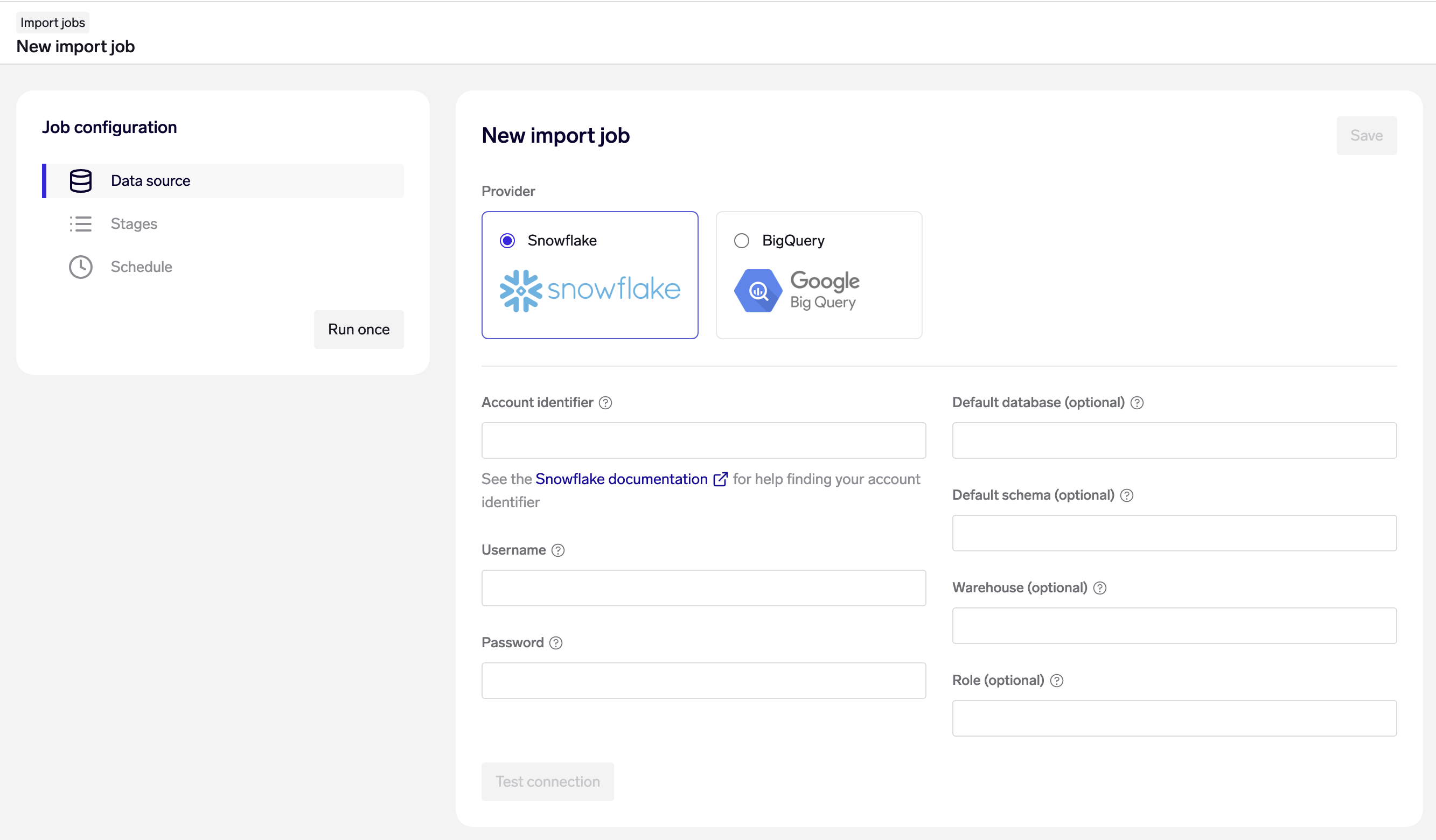
The first step is to configure a data source for your Import Job. Import jobs currently supports the following data sources:
Snowflake
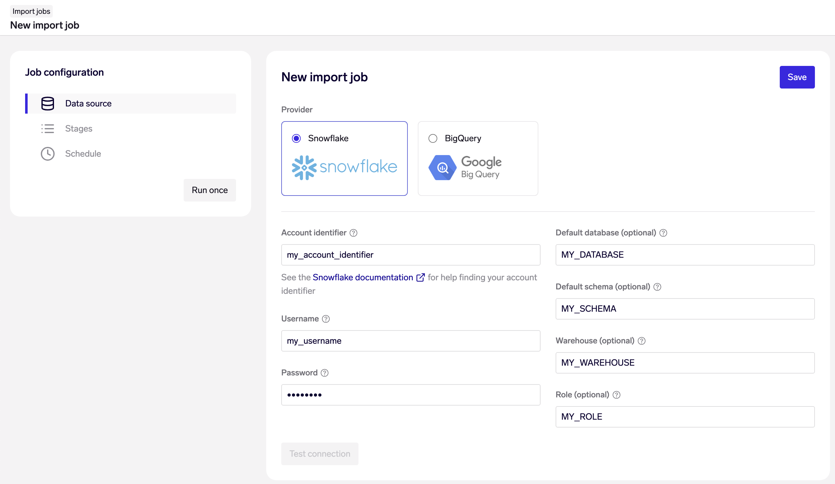
Setting up an Import Job with Snowflake credentials
On the "Data source" page of your Import Job, choose Snowflake as your data source, and fill in your account credentials and connection details:
- Snowflake account identifier: See the Snowflake documentation for help finding your account identifier.
- Snowflake username & password
- Default database & schema: optional - you may alternatively configure your Snowflake user with a default database & schema, or write your SQL queries with fully qualified table names.
- Snowflake warehouse & role: optional - you may alternatively configure your Snowflake user with a default warehouse & role.
Note: Using SQL CALL statements to stored procedures are not supported for Snowflake.
Google BigQuery
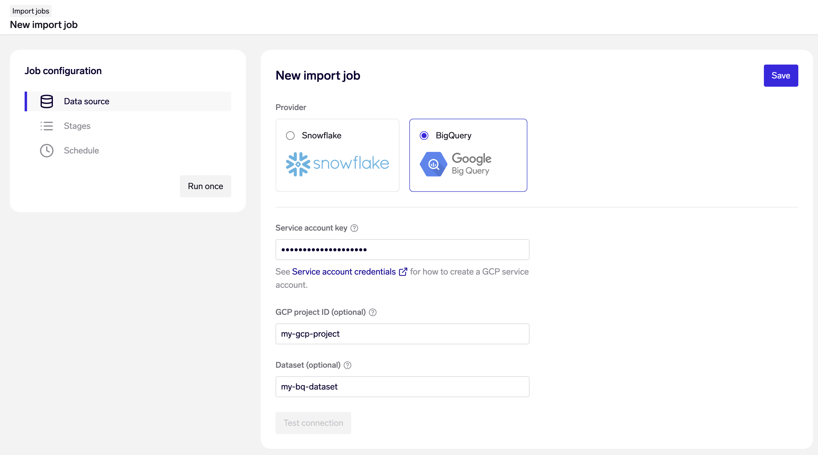
Setting up an Import Job with Google Cloud Platform service account with BigQuery access
On the "Data source" page of your Import Job, choose Google BigQuery as your data source, and fill in your account credentials and connection details:
- Service account key: The service account key (in JSON format) to authenticate with. See Service account credentials for how to create a GCP service account. The key needs to have the following permissions:
bigquery.jobs.create,bigquery.readsessions.create,bigquery.readsessions.getData,bigquery.tables.getData. - GCP project & Dataset: optional - You may alternatively write your SQL queries with fully qualified table names, e.g.
SELECT my_column FROM my_project.my_dataset.my_table as table WHERE ...
Stages
Next, create the “stages” within an Import Job. Each stage may import either entities, relationships, or time series. A stage consists of a SQL query to retrieve data, and settings for the import.
You may import complex data sets with multiple levels of granularity (e.g. data at company-level and brand-level) by creating multiple stages for the different entities, relationships and time series in your data model.
The order in which stages are executed is described below, under Running an Import Job.
Best practice for configuring stagesTypically, if accessing alternative data via Snowflake, you will have both historical data and live data in the same database tables, in the same schema. The SQL queries to retrieve both historical and live data can therefore be similar or identical.
We recommend that you plan your data import in 2 phases:
- Historical import
- Live data import
The primary differences in how your Import Job should be configured are:
- Time series stages: historical data should be loaded with either known-times for each data point, or by specifying a known-time offset; whereas live data should generally be loaded with the known-time set to the job run time (see below).
- SQL queries: historical imports should make sure to return the entire data set in the SQL query; whereas live imports should query only for recent data points that may have been added or revised. (Note: you may also choose to continue querying for the entire data set in your live pipeline, but that will cause you to incur more Snowflake costs and cause your Import Job to run slower.)
Depending on your preference, you may decide to split the historical and live data imports into 2 separate Import Jobs. Alternatively, you may build a single Import Job, run the historical import once, then modify it for live imports and schedule that on an ongoing basis.
Importing entities
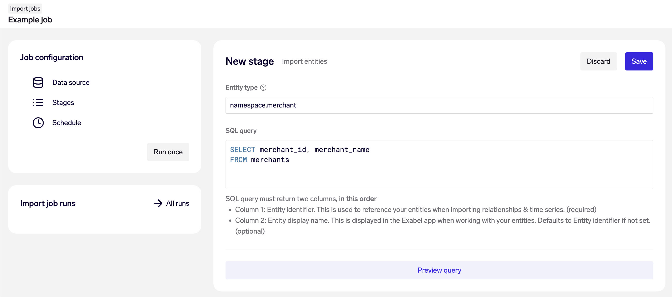
Example: Import merchants from the merchantstable
Specify the entity type that is being imported. This entity type must already be created - use this Data API endpoint if you have not done this yet.
Next, provide a SQL query that returns 2 columns - The first column should be each entity's resource name, and the second column its display name.
Entity imports are always run in upsert mode - if an entity already exists, it will be updated - so that you can run the same query and stage repeatedly in a live data pipeline.
Best practice for importing entitiesEntity resource names should be stable and consistent identifiers over time. If an entity changes display name, this should not result in a new entity being created in the data model. It is therefore important to be mindful when choosing a field as the
entitycolumn in your data source.
Importing relationships
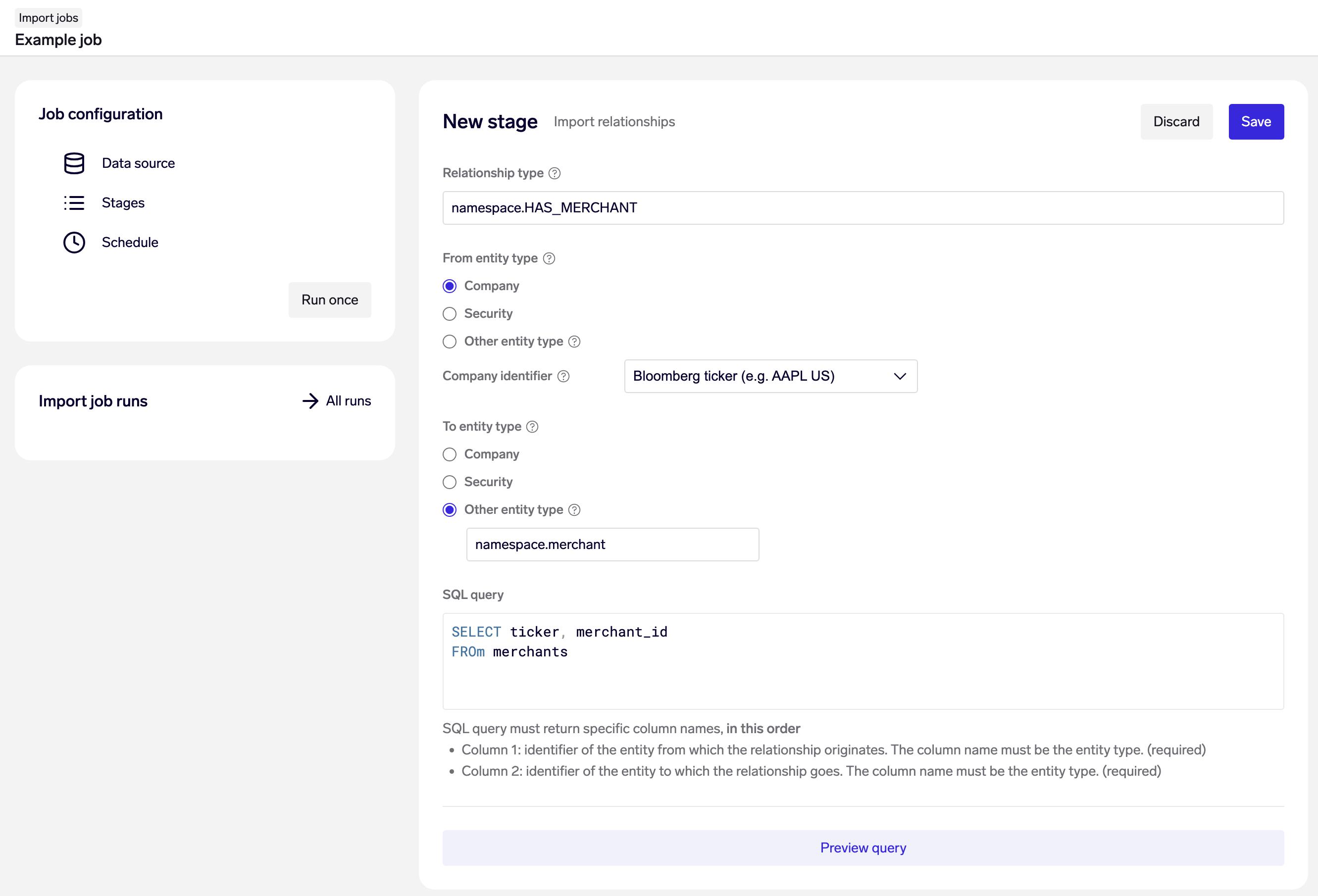
Example: Import relationships from companies to merchants from the merchantstable, looking up companies by their Bloomberg ticker.
Specify the relationship type that is being imported and the entity type of the entities that are being connected. This relationship type must already be created - use this Data API endpoint if you have not done this yet. The entities must also already exist in the data model. If entities are being mapped to or form companies or securities, specify the identifier type to be used for mapping to the companies.
Next, provide a SQL query that returns 2 columns, with the 1st column specifying the resource name of the from-entity, and the 2nd column being the resource name of the to-entity. Note: the column order here is important as it defines the direction of the relationships.
Relationship imports are always run in upsert mode - if an relationship already exists, it will be updated - so that you can run the same query and stage repeatedly in a live data pipeline.
Importing time series
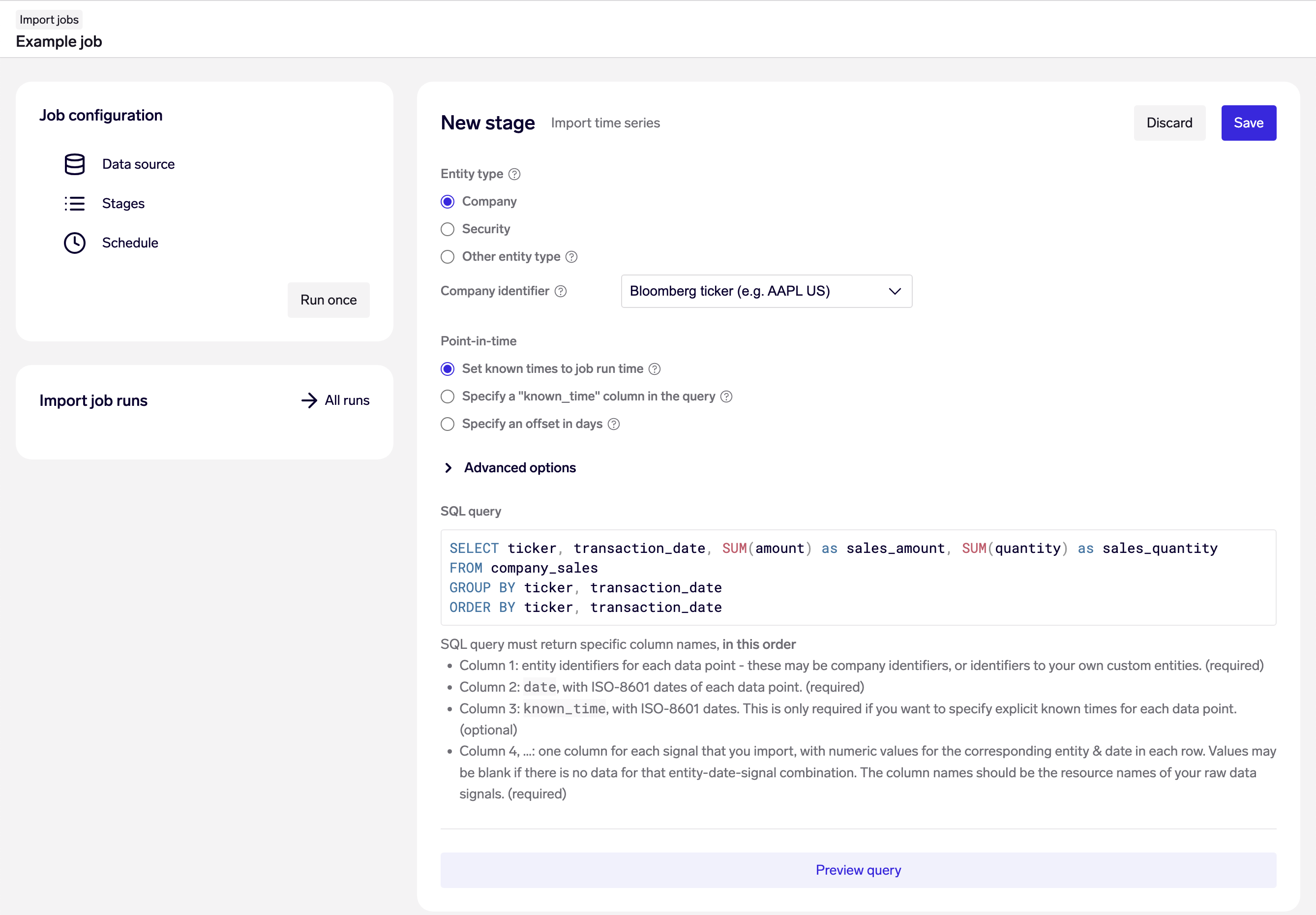
Example: Import time series for the signals sales_amount and sales_quantity on a company level from the company_salestable, looking up companies by their Bloomberg ticker.
Specify the entity type of the time series being imported. The entities must already exist in the data model. If importing entities on the company or security level, specify the identifier type to be used for mapping to the companies.
Next, choose from one of the 3 point-in-time options for determining known time on your time series data. This is important and used to avoid look-ahead bias when analyzing data.
There are 3 options for specifying known times:
- Provide data with an additional
known_timecolumn (recommended for historical backloads) - Specify an offset of 0-30 days, applied to the date of each data point (recommended for historical backloads)
- Set the known time to be the import run time (recommended for live production pipelines)
Next, specify if we should automatically create missing raw data signals. If this option is unchecked, you must make sure that you have already created the raw data signals for all time series you upload in this stage.
Finally, provide a SQL query that returns specific columns, in a specific order:
- Column 1: entity identifiers for each data point - these may be company identifiers, or identifiers to your own custom entities. (required)
- Column 2:
date, with ISO-8601 dates of each data point. (required) - Column 3:
known_time, with ISO-8601 dates. This is only required if you want to specify explicit known times for each data point. (optional) - Column 4, …: one column for each signal that you import, with numeric values for the corresponding entity & date in each row. Values may be blank if there is no data for that entity-date-signal combination. The column names should be the resource names of your raw data signals. (required)
Performance best practiceFor time series SQL queries that return in excess of 100K rows it is strongly recommended to add an
ORDER BYclause on the entity identifier and date columns (see example in screenshot above).
Importing time series on the global entity
It is also possible to connect time series to the "global" entity by setting the entity type to global and providing a SQL query that returns these specific columns:
- Column 1:
date, with ISO-8601 dates of each data point. (required) - Column 2:
known_time, with ISO-8601 dates. This is only required if you want to specify explicit known times for each data point. (optional) - Column 3, …: one column for each signal that you import, with numeric values for the corresponding entity & date in each row. Values may be blank if there is no data for that entity-date-signal combination. The column names should be the resource names of your raw data signals. (required)
Best practice for global time seriesThink carefully before loading time series to the global entity, are the raw signals truly global for your use case? If you find yourself loading multiple signals like
sales_europe,sales_americas,sales_africaand so on, you should probably introduce a region entity type with regions (Europe, Americas, Africa) as entities, and load the time series to asalessignal on these entities instead. See data modelling for more examples.
Importing time series metadata
Currency codes can be imported as time series metadata. When a currency is set on a time series, the Exabel platform will display the currency in charts, and it is possible to convert the values to another target currency without specifying the source currency.
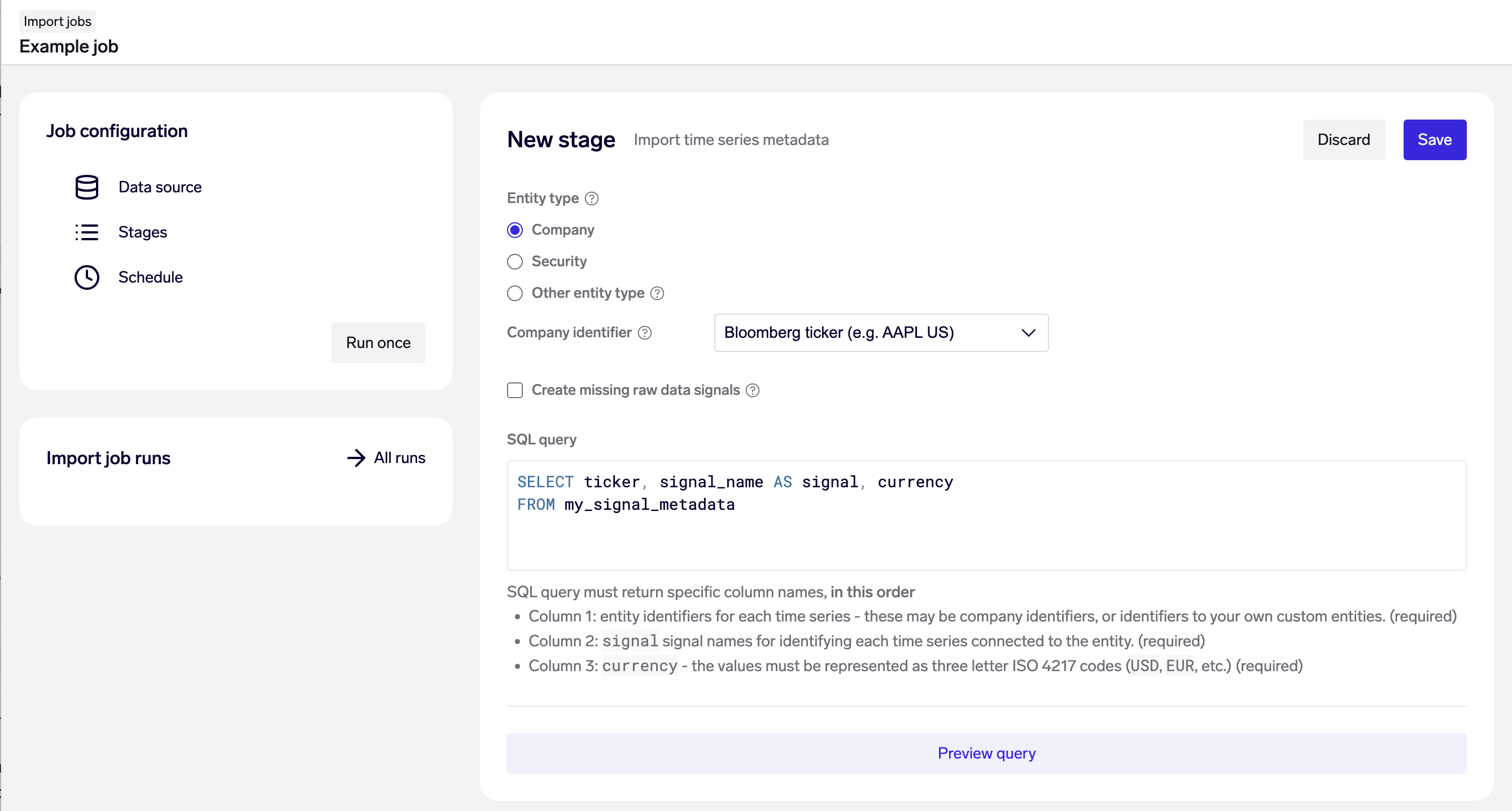
Example: Import time series metadata on company level time series, looking up companies by their Bloomberg ticker.
Specify the entity type of the time serie metadata being imported just as for regular time series data. The entities must already exist in the data model. If importing entities on the company or security level, specify the identifier type to be used for mapping to the companies.
Next, specify if we should automatically create missing raw data signals. If this option is unchecked, you must make sure that you have already created the raw data signals for all time series you upload in this stage.
Finally, provide a SQL query that returns 3 columns, in a specific order:
- Column 1: entity identifiers for each data point - these may be company identifiers, or identifiers to your own custom entities. (required)
- Column 2:
signal, signal names for identifying each time series connected to the entity. (required) - Column 3:
currency, with currency codes as three letter ISO 4217 codes in uppercase (USD, EUR, etc.). (required)
Change currency codeChanging the currency code after is it set on a time series is not supported, as it is undefined what should be done with any imported values. To change the currency of a time series, the time series must first be deleted using the Data API or Exabel SDK. See Data API or Importing via Exabel SDK.
Running an Import Job
At any point, you may run your Import Job once by clicking on the "Run once" button on the sidebar. This will trigger a new run, which you may then track on the sidebar, or by clicking into "All runs".

The "Run once" button and list of recent runs on the sidebar
Alternatively, when editing a stage, you may run that stage by clicking on the ⋮ menu on the stage, and then "Run stage once".
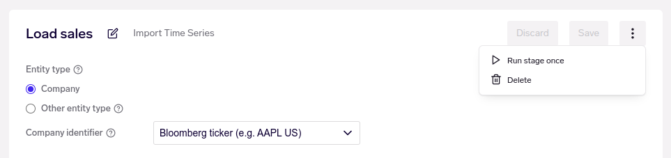
The "Run stage once" button in the stage menu
Order of execution
When running an Import Job, we try to maximize speed by executing stages in parallel where possible:
- First, all entity import stages are run in parallel, as these do not depend on each other
- Secondly, all relationship and time series import stages are run in parallel, as these depend only on entities
Therefore, the order in which your stages are listed in your Import Job does not matter.
Schedule
You can instantly turn an Import Job into a live data pipeline by going to the “Schedule” tab to schedule recurring job runs.
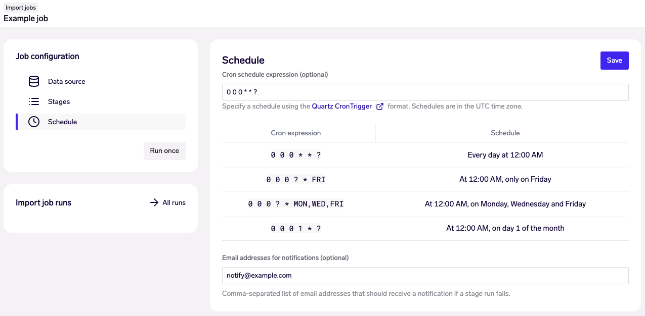
Scheduling an Import Job to run daily at Midnight UTC
Import Jobs uses the Quartz scheduler, which utilizes the cron syntax for specifying schedules. A few examples are provided in the user interface, but you may refer to the Quartz documentation for more details.
Scheduling limitsAll schedule times are specified in UTC.
Schedules may not be configured to be more often than once per hour.
Email notification of failed jobs
On the page for scheduling the job, it is possible to add a list of email addresses that will get a notification in case of a stage run fails. Note that also failure of manual runs (using the "Run once") button will be notified. If more than one stages fail, only the first stage to fail is reported.
Run status and logs
You may view the latest runs on the sidebar, as shown previously. From the sidebar, you may click on "All runs" to view all historical runs on a single page, with their start time, duration, and status.

Viewing all runs
You may then click on a particular run to view the same details at stage-level. This view also provides access to logs per stage, to aid in troubleshooting.

Viewing stages within a single run
Updated about 2 months ago