Prediction Models

Choose the right model

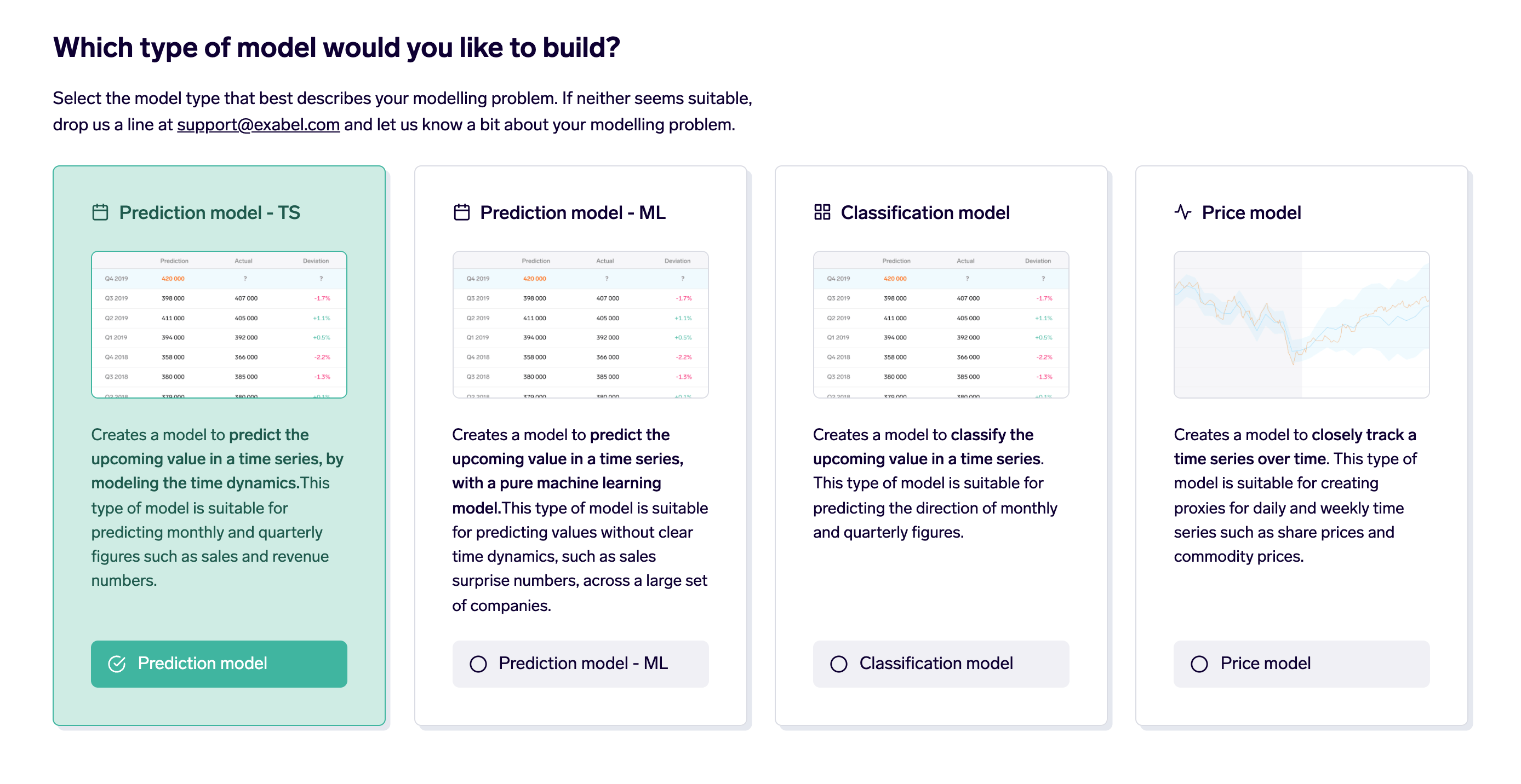
Exabel offers 4 different types of models, depending on your goal and the type of data you want to model:

Prediction model - TS (time series)
Prediction model - ML (machine learning)
Classification model
Price model

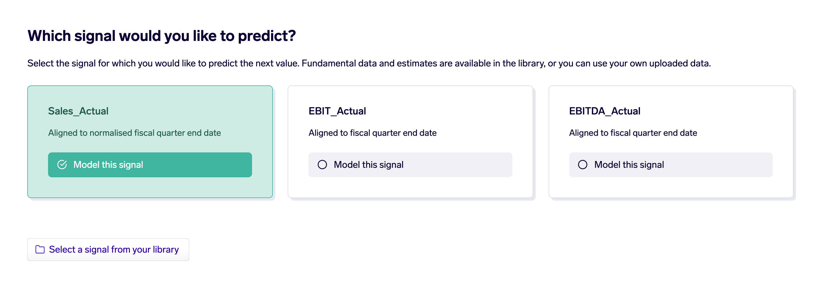
Pick the target signal

We start by identifying a target metric - what we wish to predict.

Let’s take the example of predicting a company's quarterly revenue. We can choose to predict the absolute value of revenue, or a transformed metric such as a YoY sales. Unless the input metrics are a direct explanation for sales (dollar amount), using a transformation is advised. For instance, we can use QoQ, YoY or a sales surprise metric. In either of these cases, it is ideal to include what consensus is saying the value of the target metric could be (if possible). Information that is widely available should either be included as a benchmark to measure our model against, or in the form of a surprise metric where we are then trying to predict what we can contribute over and above what the Street is saying.

Choose your universe

Next we decide what universe we wish to make a prediction for.

We should try to include all the companies for which it makes logical sense to predict the value. For example, if we are predicting same-store sales, it makes sense to include companies which sell consumer goods through stores like Nike, Adidas, Farfetch but not Facebook or Google, even if we have the relevant target and input metrics for them. Models can be trained more effectively with more data across multiple companies, and over a longer period of time.

Choose your input signals

This automatically leads us to deciding the Input metric(s) we have ahead of time that we want to use to make the prediction for a value that will be reported in future. These can be data vendor specific metrics, e.g. sales through stores, online sales, discounts offered, sentiment scores gathered through surveys or web scraped from blogs. Anything that we believe has explanation power for our choice of target metric. A good practice is to quickly check historic correlation between input and target metrics. Higher correlations are indicative of better predictive power across different machine learning models. Another key action would be to transform our input metrics on similar lines to our target metrics. Knowing the characteristics and distribution of our input data will help us in determining which type of model is better suited and also if we need further cleaning/transformation like clipping the outliers or discretizing the data. We also have the option to force a “monotone” feature on any input metric. This makes sure that we only have a positive relationship between input and target metrics (higher the input, higher the target value would be).

Our choice of model and parameters will choose which input metrics get included in the model. We always try to minimize the error by training across the flexible features and finding the best fit with least absolute or relative error. At this point, if we have chosen a benchmark signal, it provides us with a benchmark error to measure our model against.

Configure modelling technique

There are few steps involved in making a choice for our modelling technique:

Step 1: Choosing panel vs independent models

A panel model has more pairs of (input, target) as it disregards the company label and pools in all the data to train on. So if we have less historic data, the panel model is an ideal choice. Since the data is company-agnostic it needs to be more comparable to make sense out of it. This encourages us to look into distribution of our input metrics (e.g. min, max, 3 Ms, standard deviation) and make it more uniform. If we have too much variation in input metrics per company and intend to use them as is, an independent model is a better choice. The model then tries to find the best set of parameters for each company separately. Panel model can be considered more robust as it reduces the chances of over-fitting for each company separately. Given the same performance, it would be the ideal choice.

Side-note: As feedback from the model runs, if we don’t see good results but are convinced with our logic, we should try establishing a better relationship between input and target metrics. Few steps that are suggested - check distribution, normalise outside the model, clip/truncate extreme values, discretise inputs, handle inflection points or outliers in the data etc

Step 2: Normalising data independently vs across all companies

This should be decided based on characteristics of our data and what information loss would it bring choosing one over the other and if it is desired. In general, if the data is on the same scale across different companies, such as when the data represents YoY percentage changes, it is advisable to normalise across all companies. On the other hand, if the scale is vastly different, such as for revenue numbers which can be orders of magnitude larger for one company versus another, it is advisable to normalise the data separately per company.

Step 3: Choosing the ML model

We can leave it at the default choice of Auto, which means that a few model types (such as Elastic Net, Neural Networks and Extreme Gradient Boosting) will be tested to determine what works best for this particular data set. Alternatively, a specific model type can be specified. This choice is easier if we have an idea on the linear vs non-linear relationship between target and input metrics. If we know or expect it to be linear, Elastic Net is a good choice. If non-linear, then we first try with the Extreme Gradient Boosting model, or alternatively a Neural Network. Understanding what these models individually mean and do can help in fine tuning the parameters, else we go ahead with our default options. We provide several other options in our model technique suite, like Decision Tree or Huber Regression.

If “independent models for each company” was selected, then it’s also possible to run classical statistical time series models, such as SARIMAX or Unobserved Components. These can be used with or without input variables. Without input variables, this is called Univariate modelling. Such modelling can be used e.g. for forecasting intra-quarter values and using them to fill the remaining quarter (substitute to extrapolation). We can use e.g. the modelling technique “unobserved component” for it with the Autoregressive option enabled.

Step 4: Walk forward vs cross validation

We can choose to do a walk forward approach where we keep adding each data point in our time series and make the next prediction on expanding the window of data. Or we choose to do an n-fold cross validation to test/train the model, where the companies are divided into 5 folds, and we make predictions for each fold by training a model on the data from the other 4 folds. The advantage of the walk forward backtesting is that we see predictions as they would have been made at that time, since only prior data is used for training the model. The advantage of cross validation is that all the tested models have been trained with about 80% of the data, spread throughout time, which can be helpful when there are different time regimes, such as pre- and post covid.

Step 5: Choosing parameters

Ensemble model: By default, the system will combine several models into an ensemble model, if that is seen to give better results in the backtests. By checking the box, this feature will be disabled, and only the single best-performing model will be used as the final model.
Lags: If the chosen value is not zero, the model will include lagged versions of all input signals as additional inputs to the model (including the target signal, if the model is auto-regressive). If we only want lagged versions for some of the input signals, then this setting should be set to 0, and we can add separate input signals that have been manually lagged through the DSL expression.
Seasonality: Enable if target has a seasonality component e.g. quarterly revenue, but not needed if we already did the YoY transformation (which effectively removes seasonality)
Linear trend: When turned on, the linear trend will be calculated for all input signals (including the target signal if the model is auto-regressive) and used as additional inputs to the model. The linear trend is defined as the growth rate over the past 5 data points, and is calculated by running a regression over these past data points with time as the regressor (the coefficient from the regression is then taken as the trend).
Auto-regressive: If enabled, includes the previous value(s) of the target signal as additional inputs to the model.
Hyperopt level: Enabled if we want the system to search for the best settings (choice of model type, which inputs to use, whether to include seasonality and lags, and so on). The higher the hyperopt level, the more combinations of settings are attempted, and thus increases the run time, as well as the risk of overfitting, but also gives the system a better chance to find a good combination of settings.